ELS: a latency-based load balancer, part 2

December 9, 2015 Published by Lukáš Poláček

What to Measure?

In part 1, we already mentioned a few metrics that should be considered by the load balancer.

Success latency ℓ and success rate s of each machine.
Number of outstanding requests q between the load balancer and each machine. These are the requests that have been sent out but haven’t received a reply yet.
Fast failures are better than slow failures, so we also measure failure latency f for each machine.

In addition, parallelism p is useful. Some machines might have more processors, better memory, etc., allowing them to work on more requests in parallel. It’s important to measure parallelism and not just rely on the number of processors reported by the machine, since they might be occupied by other processes and thus not available to the service we are interested in.

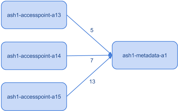
We also note that we only use locally available information. There are other load balancers sending requests to the same machine, but we don’t take them into account when calculating the number of outstanding requests.

Sharing the number of outstanding requests between different load balancers is useful, but it also comes at a cost of much higher code complexity. Another disadvantage is that when a load balancer broadcasts its load to others, that information becomes immediately obsolete, since requests come and go within milliseconds. There is no now in distributed systems.

How to Measure It?

A commonly used measuring method is exponentially moving weighted average. We employ a similar method called forward exponential decay, inspired by Forward Decay: A Practical Time Decay Model for Streaming Systems by Cormode et al.

The exponential decay is determined by the time bias parameter. When the time bias is set to 1 minute, about 63.2% of the value is coming from the last minute measurements, 23.3% from the minute before that (0.233 = (1 – 0.632) * 0.632), etc. The weight is decreasing exponentially with each passing minute, historical data older than t minutes have weight 1 / exp(t). The most recent minute has weight 63.2%, since 63.2% = 1 – 1 / exp(1). Unix load average is calculated similarly.

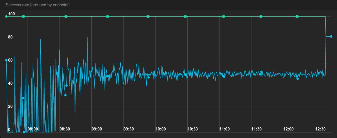
If you set the time bias too low, the measurements will be noisy and will jump up and down a lot. Below is a graph of measured success rate in a benchmark similar to the second benchmark presented in part 1. One machine has 50% success rate while all others have perfect 100%.

In the beginning of the benchmark the traffic was too low, so there were too few requests in each time bias window and therefore the measured success rate was jumping up and down a lot. The measurements became much more stable once the rate of requests went up.

On the other hand, if you set the time bias too high, the load balancer wouldn’t notice sudden increase in latency until it’s too late.

To get around this problem, we also provide an option to make the time bias adapt to the current rate of traffic. Users can set desired rate and the load balancer will make sure that each machine is expected to get that many requests in a single time bias window. Thus the time bias shouldn’t be too low or too high.

Expected Latency from User’s Perspective

In part 1 we mentioned that we calculate the expected latency from user’s perspective based on all gathered metrics.

Suppose a machine has success rate of 50%. With probability 1/2 we need to do the first retry, with probably 1/4 we also need to do a second retry, etc. In total, we need 1 + 1/2 + 1/4 + 1/8 + 1/16 + … = 2 tries for one correct response. This means that on average 1 request fails and 1 succeeds, so we expect to wait ℓ + f ms for a successful response (recall that ℓ is success latency and f is failure latency). In general, success rate s leads to 1 / s tries on average (see geometric distribution).

We take into account round-trip time back to the Spotify client when the client retries after a failure. Being pessimistic, we assume that it’s a client on the other side of the globe with a bad connection, so the time penalty for a failure round-trip is 800 milliseconds.

In total, L = ℓ + (f + 800)(1 / s – 1) ms is the expected arrival time of a correct response, assuming there are no other requests waiting to be processed.

Side note: as explained in Google’s paper The Tail at Scale, for services that trigger many more requests downstream in the backend, even one bad or slow reply causes a lot of problems. The formula presented above does not represent such case very well. Perhaps a carefully configured relative circuit breaker should be employed instead.

Spotify clients also do exponential back-off when retrying, but for simplicity this is not taken into account and it wouldn’t change the result a lot anyway.

Assuming only one processor, with latency L and q outstanding requests, we should wait L * (q + 1) ms for a reply, because there are q + 1 requests to process in total. With p processors, we get L * (q / p + 1) ms.

Instead of the number of processors, we should use the rate of parallelism as observed by the load balancer, as we previously discussed. We tried it and unfortunately the performance got worse. We don’t have a good explanation for that. Possible explanations include:

We used a bad measurement method for the rate of parallelism.
Perhaps parallelism is already accounted for, because queue size decreases faster for highly parallel machines.

Since adding parallelism to the formula didn’t help, we ended up using E = L * (q + 1) ms as the expected latency.

Convert Expected Latency to Weight

Suppose we have three one-core machines with latencies 10 ms, 20 ms, and 50 ms. There’s 1000 milliseconds in one second, so they can handle 100, 50 and 20 requests per second respectively.

It makes sense to send traffic using ratio 10:5:2, since that’s proportional to their speeds. The load balancer is probabilistic and 7.2 times higher weight means 7.2 times higher chance of getting a request. Therefore we choose the weight to be 1 / E, where E is the computed expected latency (E = L * (q + 1) = (ℓ + (f + 800) * (1 / s – 1)) * (q + 1)). The lower the latency, the higher the speed and the higher the weight.

It should be noted that the optimal proportion is different when the system is not saturated. When the traffic is very low, the fastest machine might be able to handle all the traffic. However, this is yet another place where we would need to share information between hosts and we don’t want to do that for reasons mentioned earlier.

Improving Tail Latency

Inspired by C3 for Cassandra, we have tweaked the formula a bit to 1 / L / (q + 1)³, where L is the computed expected latency. This formula leads to better tail latency (the 99th percentile), since it punishes machines that have too many outstanding requests.