How Spotify Optimized the Largest Dataflow Job Ever for Wrapped 2020
In this post we’ll discuss how Spotify optimized and sped up elements from our largest Dataflow job, Wrapped 2019, for Wrapped 2020 using a technique called Sort Merge Bucket (SMB) join. We’ll present the design and implementation of SMB and how we incorporated it into our data pipelines.
Introduction
Shuffle is the core building block for many big data transforms, such as a join, GroupByKey, or other reduce operations. Unfortunately, it’s also one of the most expensive steps in many pipelines. Sort Merge Bucket is an optimization that reduces shuffle by doing work up front on the producer side. The intuition is that for datasets commonly and frequently joined on a known key, e.g., user events with user metadata on a user ID, we can write them in bucket files with records bucketed and sorted by that key. By knowing which files contain a subset of keys and in what order, shuffle becomes a matter of merge-sorting values from matching bucket files, completely eliminating costly disk and network I/O of moving key–value pairs around. Andrea Nardelli carried out the original investigation on Sort Merge Buckets for his 2018 master’s thesis, and we started looking into generalizing the idea as a Scio module afterwards.
Design and Implementation
The majority of the data pipelines at Spotify are written in Scio, a Scala API for Apache Beam, and run on the Google Cloud Dataflow service. We implemented SMB in Java to be closer to the native Beam SDK (and even wrote and collaborated on a design document with the Beam community), and provide Scala syntactic sugar in Scio like many other I/Os. The design is modularized into the main components listed below — we’ll start with the two top-level SMB PTransforms — the write and read operations SortedBucketSink and SortedBucketSource.
SortedBucketSink
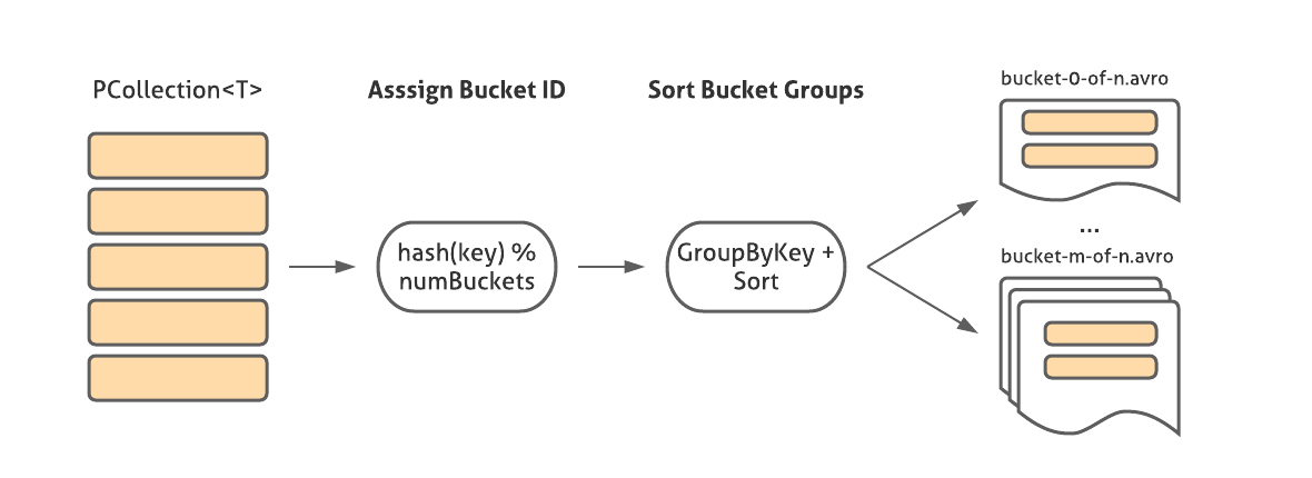
This transform writes a PCollection (where T has a corresponding FileOperations instance) in SMB format. It first extracts keys and assigns bucket IDs using logic provided by BucketMetadata, groups key–values by the ID, sorts all values, and then writes them into files corresponding to bucket IDs using the FileOperations instance.
In addition to the bucket files, a JSON file is also written to the output directory representing the information from BucketMetadata that’s necessary to read the source: the number of buckets, the hashing scheme, and the instructions to extract the key from each record (for example, for Avro records we can encode this instruction with the name of the GenericRecord field containing the key).
SortedBucketSource
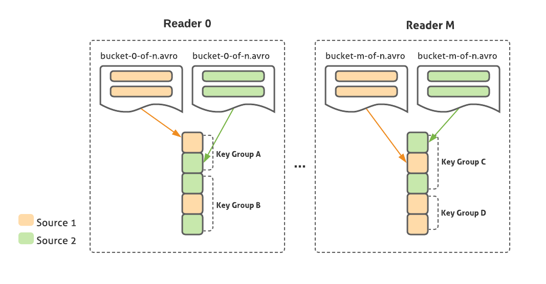
This transform reads from one or more sources written in SMB format with the same key and hashing scheme. It opens file handles for corresponding buckets from each source (using FileOperations for that input type) and merges them while maintaining sorted order. Results are emitted as CoGbkResult objects per key group, the same class Beam uses for regular Cogroup operations, so the user can extract the results per source with the correct parameterized type.
FileOperations
FileOperations abstracts away the reading and writing of individual bucket files. Since we need fine-grained control over the exact elements and their order in every file, we cannot leverage the existing Beam file I/Os, which operate on a PCollection level and abstract away the locality and order of elements. Instead, SMB file operations happen at a lower level of BoundedSource for input and ParDo for output. Currently Avro, BigQuery TableRow JSON, and TensorFlow TFRecord/Example records are supported. We plan to add other formats like Parquet as well.
BucketMetadata
This class abstracts the keying and bucketing of elements, and includes information such as key field, class, number of buckets, shards, and hash function. The metadata is serialized as a JSON file alongside data files when writing, and used to check compatibility when reading SMB sources.
Optimizations and Variants
Over the last year and a half we’ve been adopting SMB at Spotify for various use cases, and accumulated many improvements to handle the scale and complexity of our data pipelines.
Date partitioning: At Spotify, event data is written to Google Cloud Services (GCS) in hourly or daily partitions. A common data engineering use case is to read many partitions in a single pipeline — for example, to compute stream count over the last seven days. For a non-SMB read, this can be easily done in a single PTransform using wildcard file patterns to match files across multiple directories. However, unlike most File I/Os in Beam, the SMB Read API requires the input to be specified as a directory, rather than a file pattern (this is because we need to check the directory’s metadata.json file as well as the actual record files). Additionally, it must match up bucket files across partitions as well as across different sources, while ensuring that the CoGbkResult output correctly groups data from all partitions of a source into the same TupleTag key. We evolved the SMB Read API to accept one or more directories per source.
Sharding: Although the Murmur class of hash functions we use during bucket assignment usually ensures an even distribution of records across buckets, in some instances one or more buckets may be disproportionately large if the key space is skewed, creating possible OOM errors when grouping and sorting records. In this case, we allow users to specify a number of shards to further split each bucket file. During the bucket assignment step, a value between [0, numShards) is generated randomly per bundle. Since this value is computed completely orthogonally to the bucket ID, it can break up large key groups across files. Since each shard is still written in sorted order, they can simply be merged together at read time.
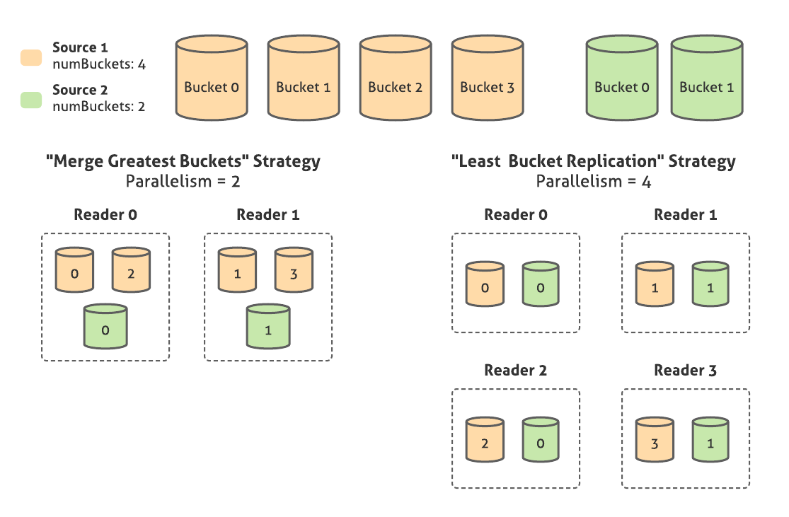
Parallelism: Since the number of buckets in an SMB sink is always a power of 2, we can come up with a joining scheme across sources with different numbers of buckets based off of a desired level of parallelism specified by the user. For example, if the user wants to join Source 1 with 4 buckets and Source 2 with 2 buckets, they can specify either:
Minimum parallelism, or “Merge Greatest Buckets” strategy: 2 parallel readers will be created. Each reader will read 2 buckets from source A and 1 from source B, merging them together. Because bucket IDs are assigned by taking the integer hash value of the key modulo the desired number of buckets, mathematically we know that the key spaces of the merged buckets overlap.
Maximum parallelism, or “Least Bucket Replication” strategy: 4 parallel readers will be created. Each reader will read 1 bucket from Source A and 1 from Source B. After merging each key group, the reader will have to rehash the key modulo the greatest number of buckets, to avoid emitting duplicate values. Therefore, even though this strategy achieves a higher level of parallelism, there is some overhead of computing duplicate values and rehashing to eliminate them.
Auto parallelism: Creates a number of readers between minimal and maximal amounts, based on a desired split size value provided by the Runner at runtime.
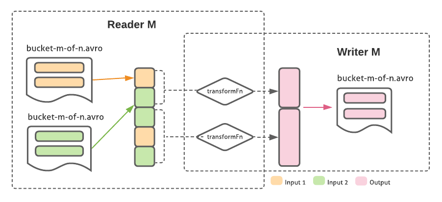
SortedBucketTransform: A common usage pattern is for pipelines to enrich an existing dataset by joining it with one or more other sources, then writing it to an output location. We decided to specifically support this in SMB with a unique PTransform that reads, transforms, and writes output using the same keying and bucketing scheme. By doing the read/transform/write logic per bucket on the same worker, we can avoid having to reshuffle the data and recompute buckets — since the key is the same, we know that the transformed elements from bucket M of the inputs also correspond to bucket M in the output, in the same sorted order as they were read from.
External Sort: We made a number of improvements to Beam’s external sorter extension, including replacing the Hadoop sequence file with the native file I/O, removing the 2GB memory limit, and reducing disk usage and coder overhead.
Adoption — Core Data Producers
Since SMB requires data to be bucketed and sorted in a specific fashion, the adoption naturally starts from the producer of that data. A majority of the Spotify data processing relies on a few core data sets that act as single sources of truth for various business domains like streaming activities, user metadata and streaming context. We worked with the maintainer of these data sets to convert a year’s worth of data to SMB format.
Implementation was straightforward since SortedBucketSink is mostly a drop-in replacement for the vanilla Avro sink with some extra settings. We were using Avro sink with the sharding option to control the number and size of output files. After migrating to SMB, we did not notice any major bump in terms of vCPU, vRAM, or wall time since sharding requires a full shuffle similar to the additional cost of SMB sinks. A few other settings we have since had to tweak:
Agree on user_id as a hexadecimal string as bucket and sort key, since we need the same key type and semantic across all SMB datasets.
Set compression to DEFLATE with level 6 to be consistent with the default Avro sink in Scio. As a nice side effect of data being bucketed and sorted by key, we observed ~50% reduction in storage from better compression due to collocation of similar records.
Make sure output files are backwards compatible. SMB output files have “bucket-X-shard-Y” in their names but otherwise contain the same records with the same schema. So existing pipelines can consume them without any code change; they just do not leverage the speedup in certain join cases.
Adoption — Wrapped 2020
Once the core datasets were available in SMB format, we started Wrapped 2020, building off the work left from the Wrapped 2019 campaign. The architecture was meant to be reusable and was a great place to start. However, the source of data was a large, expensive Bigtable cluster that had to be scaled further up to handle the load of Wrapped jobs. We wanted to save cost and time by moving from Bigtable to SMB sources. This year we also needed to handle new complex requirements for filtering and aggregating streams. This required us to join a large dataset containing stream contextual information to the user’s listening history. This would have been nearly impossible or at the very least extremely expensive because of the considerable size of each of these joins. Instead we tried using SMB to eliminate that join completely and avoid using Bigtable as our listening history source.
To compute Wrapped 2020, we had to read from three main data sources for streaming activity, user metadata and streaming context. These three sources had all the data we needed to generate each person’s Wrapped while filtering based on listening context. Previously, the Bigtable had 5 years’ worth of listening history already keyed by user_id. Now, we are able to read data already keyed by user_id from these three sources through SMB. We then aggregated a year’s worth of data per key to calculate each user’s Wrapped.
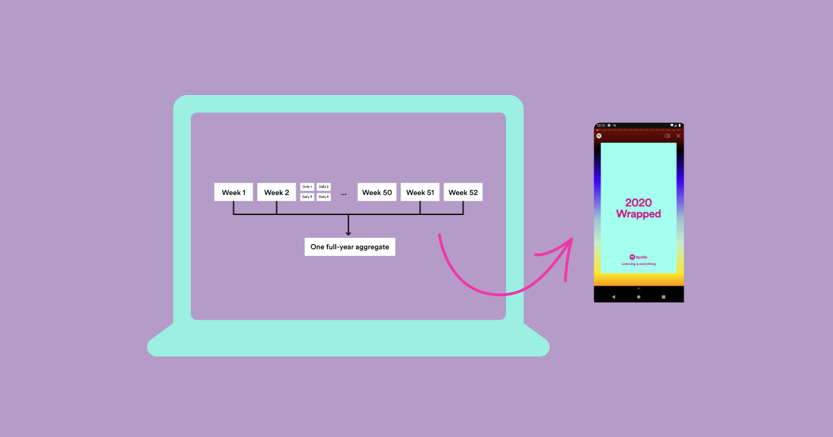
Because 1 of the 3 main sources are partitioned hourly while the other 2 are partitioned daily, it would be problematic to read a year’s worth of data in one job due to the excessive number of concurrent reads from the hourly partitioned source. Instead, we first ran smaller jobs that would aggregate a week’s or day’s worth of play counts, msPlayed, and other information on each user. From there, we then aggregated all these smaller partitions to a singular partition of data that would hold a year’s worth of data.
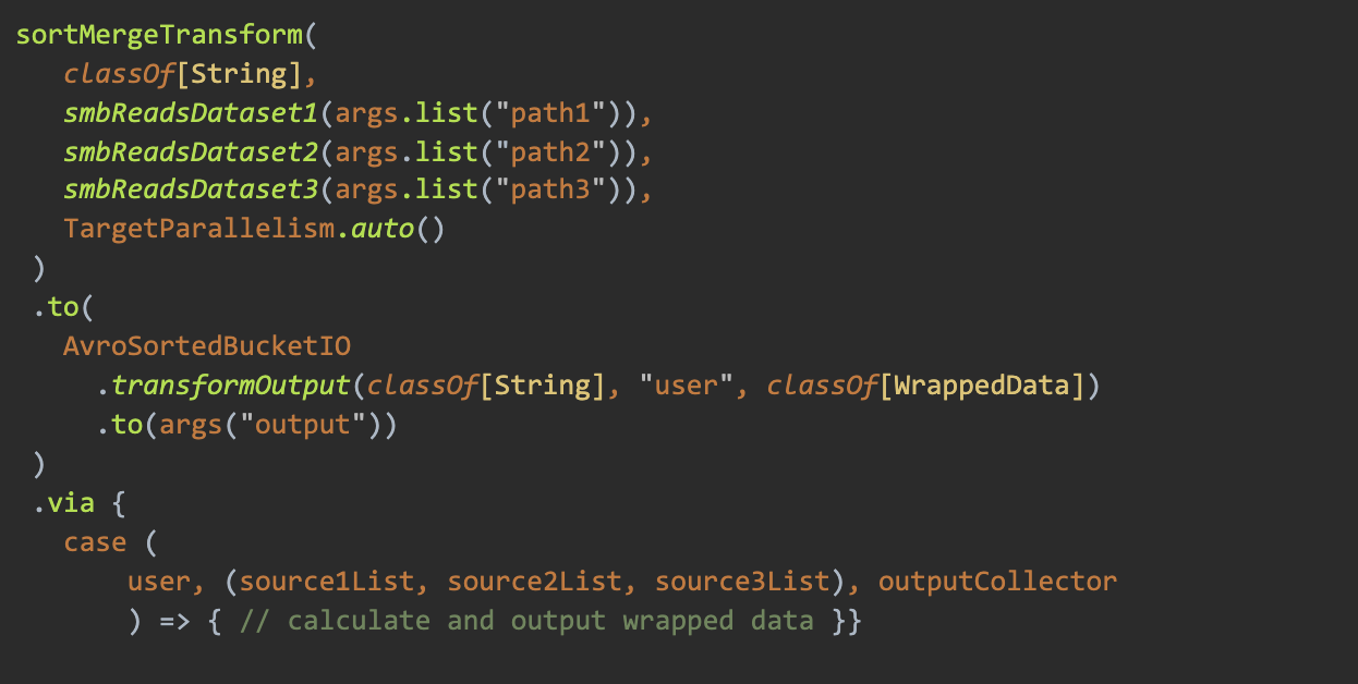
SMB made this relatively easy. We used sortMergeTransform to combine our three sources of data, read each one keyed by user_id, and write our Wrapped output (play counts, ms played, play context, etc.) in SMB format.
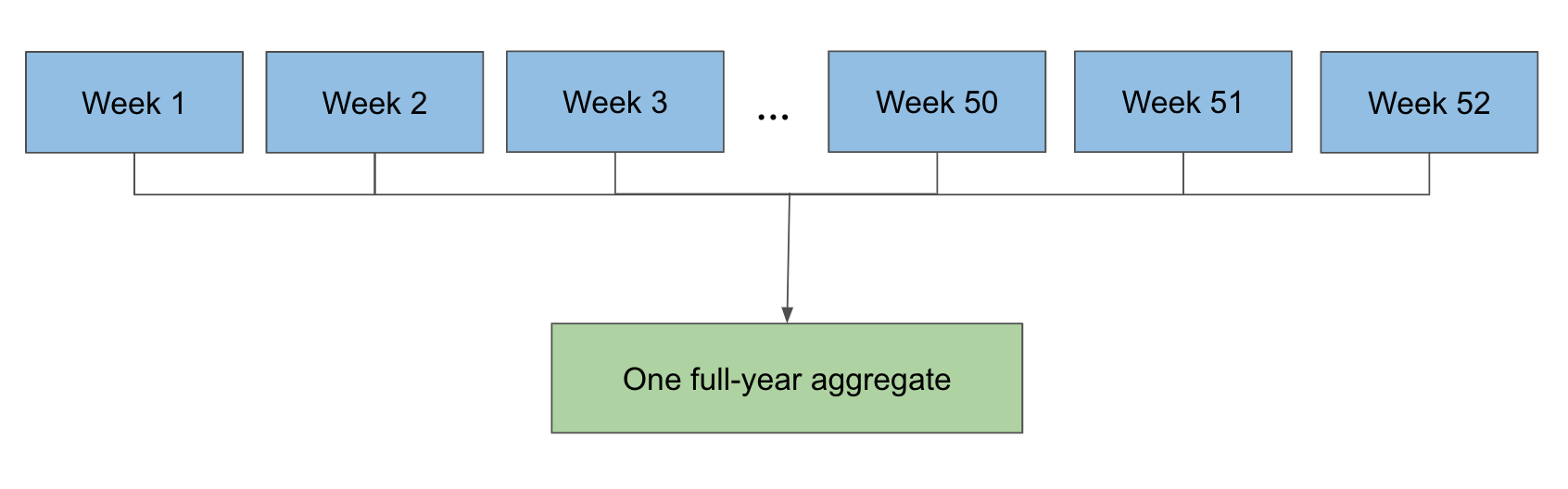
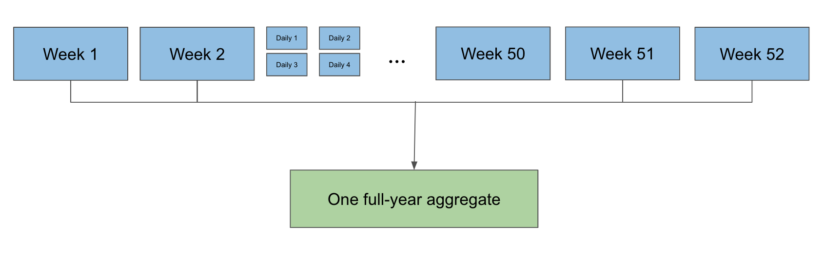
Finally, we ran our aggregate job that uses sortMergeGroupByKey to read all Wrapped weekly partitions of SMB, combine a year’s worth of data, and write the output so later jobs can calculate the rest of Wrapped. A key point of flexibility here is that the aggregate job can take any mix of weekly and daily partitions, which is incredibly helpful logistically when running these jobs. The end result in practice looks something like this:
This ended up being a huge cost savings for us in this year’s Wrapped project. By leveraging SMB, we managed to join roughly a total of 1PB data without using conventional shuffle or Bigtable. We estimate around a 50% decrease in Dataflow costs this year compared to previous years’ Bigtable-based approach. Additionally, we avoided scaling the Bigtable cluster up two to three times its normal capacity (up to around 1,500 nodes at peak) to support the heavy Wrapped jobs. This was a huge win in this year’s campaign as we were able to bring a wonderful experience in a more cost effective way than ever before.
Conclusion
By adopting SMB, we were able to perform extremely large joins that were previously either unfeasible or cost-prohibitive, or that required custom workarounds like Bigtable. We achieved significant cost savings and opened up more ways of optimizing our workflows. There’s still much work to be done. We look forward to migrating more workflows to SMB, while handling more edge cases like data skew, composite keys, and more file formats.
SHARE THIS ARTICLE