Bringing Sequential Testing to Experiments with Longitudinal Data (Part 2): Sequential Testing

In Part 1 of this series, we introduced the within-unit peeking problem that we call the “peeking problem 2.0”. We showed that moving from single to multiple observations per unit in analyses of experiments introduces new challenges and pitfalls with regards to sequential testing. We discussed the importance of being clear about the distinctions between measurement, metric, estimand, and estimator, and we exemplified those distinctions with so-called cohort-based metrics and open-ended metrics. In a small simulation, we showed that standard sequential tests combined with open-ended metrics can lead to inflated false positive rates (FPRs). 

In Part 2 of the series, we share some learnings from implementing sequential tests based on data with multiple observations per unit, i.e., so-called longitudinal data.

We cover the following topics:

• Why we need to pay extra attention to longitudinal data in sequential testing
• Practical considerations for running sequential tests with longitudinal data
• How group sequential tests (GSTs) apply to longitudinal data models, and some GST-specific aspects to be mindful of
• Some concluding remarks on how Spotify applies sequential tests on longitudinal data experiments

Why do we need to pay extra attention to longitudinal data in sequential testing?

It’s not uncommon to use longitudinal data in online experimentation, and typically this requires no special attention when using fixed-horizon analysis. However, when combining longitudinal data and sequential testing, longitudinal data quickly introduces particular challenges. To derive fixed-horizon tests for any test statistic, it’s sufficient to know its marginal sampling distribution. For sequential tests, we need to know the dependence structure of the vector of test statistics over the intermittent analyses. With one observation per unit, the dependence between test statistics only comes from the overlapping sample of independent units. With longitudinal data, the covariance between the test statistics at two intermittent analyses comes both from new measurements of the same units and the overlapping sample between the analyses. 

This might seem like a subtle difference, but for sequential testing this complicates things. We typically operate under an assumption of independent measurements between units — but not within units. The dependency within units complicates the covariance structure of the test statistics in a sequential test — which, in turn, makes it more complicated to derive valid and efficient ways of conducting sequential inference. 

Practical considerations for running sequential tests with longitudinal data 

When extending experimentation with sequential testing from cross-sectional to longitudinal data, several things change. Here, we dig into two important aspects:

1. The mental switch from “metrics” to “models”
2. The challenges of compressing data to scale result calculations across thousands of experiments 

The mental switch from “metrics” to “models”

When diving into the longitudinal data literature, it’s clear that the current view of metrics in the online experimentation community is insufficient. 

In the case of a single observation per unit, it’s often possible to have the same “metric” (e.g., a mean or sum of some aspect of a unit) in a dashboard as in an experiment. We can use the difference-in-means estimator to estimate the average treatment effect, and there is a simple and beautiful mapping between the change in our experiment and the expected shift in the dashboard metric if we roll out the A/B-tested experience to the population. 

In the case of longitudinal data with multiple observations per unit, this mapping is much harder to achieve. The open-ended metric might be a natural metric for some, but it’s not obvious how open-ended metrics map to any metric you would put in a dashboard. As we showed in Part 1 of this series, the open-ended metric is a function of the influx to the experiment, which might even be a function of the experiment’s design (rather than, for example, the natural activity of users). 

We find that it’s a good idea to simply switch mindset from “metrics” to “models” when we move over to the longitudinal data experiments. Instead of thinking about metrics and mean differences in these metrics, we think about what estimands we’re interested in, and what models and estimators we can use to estimate them robustly and efficiently. Approaching the problem from the modeling perspective means that we can use the rich literature on econometrics panel data modeling and general longitudinal data modeling to help solve our challenges. See, for example, the books Econometric Analysis of Cross Section and Panel Data and Applied Longitudinal Analysis.  

Data compression and sufficient statistics

When dealing with millions and even hundreds of millions of users in a sample, it’s inconvenient to handle raw (e.g., per unit or per measurement) data in memory on the machine performing the statistical analysis. Instead, online experimenters with large samples let data pipelines produce summary statistics that contain the information needed for the analysis. In statistics, the information from the raw data needed for an estimator is called “sufficient statistics”, i.e., a set of summary statistics that are sufficient for obtaining the estimator in question. 

For the classic difference-in-means estimators, the sufficient statistics per treatment group are the sum, the sum of squares, and the count of the outcome metric. For sequential testing, no additional information is typically needed. This means that, regardless of the sample size, the analysis part of the platform only needs to handle three numbers for each group and intermittent analysis. In other words, the size grows linearly in the number of analyses. 

With longitudinal data models, more attention is required for the within-unit covariance structure. For many models and estimators, the within-unit covariance matrix needs to be estimated or at least corrected for. Let K be the max number of measurements per person in the sample. Then estimating the covariance matrix implies that K*(K+1)/2 parameters need to be estimated. In other words, the number of sufficient statistics is increasing quadratically in K.

There are many classical statistical models that can be used for sequential testing of parameters with increasing longitudinal data. However, for many of those, the ability to compress the raw data before doing the analysis is limited — which makes their practical applicability questionable. For a nice introduction on data compression for linear models, see Wong et al. (2021).    

Longitudinal models let us use all available data at all intermittent analyses

Open-ended metrics, as defined in Part 1, are challenging from a sequential testing perspective. As we discussed in the previous section, to conduct a sequential test, we need to account for the covariance structure of the test statistics across the intermittent analyses. We will now widen our scope from open-ended metrics and talk about ways to use all available data at all intermittent analyses. The main argument of using open-ended metrics is that they allow for exactly that, but as we will show, there are many other ways to estimate treatment effects using all available data. 

Formulating what to test really comes down to trade-offs between ease of derivation and implementation of sequential tests, which population treatment effect we aim to estimate, and the efficiency of the estimator.   

How to model treatment effects with longitudinal data  

Since the data going into open-ended metrics is simply ordinary panel data, we can approach the sequential testing from that perspective. There are many ways to model and estimate parameters of interest from longitudinal data. It’s helpful for our discussion to consider the following simple model:

Here, is the unit i at measurement t under treatment d. The parameter

is the contrast between treatment and control. Depending on our estimation strategy, the estimand that we estimate with this parameter will differ.  

In principle, there are two ways of going about longitudinal data modeling: 

1. Use standard cross-sectional models for the point estimate, and use cluster-robust standard errors to deal with the within-unit dependency. This includes, for example, ordinary least squares (OLS) and weighted least squares (WLS) with robust standard-error estimators. 
2. Use a model that explicitly models the dependency structure as part of the model, for example, generalized least squares (GLS) and the method of generalized estimating equations (GEE). 

To make this concrete, we consider the following three estimators for the model above.

• ROB-OLS: Estimating with OLS and using cluster-robust standard errors 
• ROB-WLS: Estimating with WLS and using cluster-robust standard errors
• GLS: with GLS (assuming the covariance structure is known or estimated as unstructured)

This list of estimators is by no means exhaustive and was selected for illustrative purposes. The main differences between these estimators are that, first, they give different weights to different units and measurements in the point estimate and, second, they give different standard errors and therefore have different efficiency. Next, we look closer at the weights. 

Weights of units and measurements

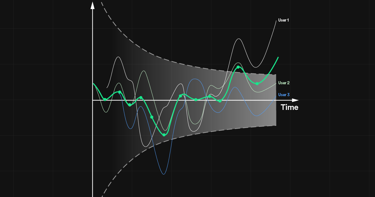
We return to the small example dataset from Part 1 of this series, in Figure 1, below. We assume data is delivered in batches. For example, this could be daily measurements being delivered after each day has passed. In this example, the observed cumulative samples at the three first batches are as follows:

Here, when the third batch has come in, the first and second units are observed three times, whereas the third and fourth units are observed twice, and the fifth and sixth units are observed only once. As a simple but illustrative data-generating process, we assume that there is a unique average treatment effect at each time point after exposure. That is, and , thus .

The weights for each measurement in the point estimator for the ROB-OLS estimator is 1/(total number of measurements in sample) for each measurement. This in turn implies that the point estimator has the expected value

.

For the ROB-WLS, the weights can be selected by the analyst. Interestingly, by selecting the weights for each unit to be 1/(number of observed measurements for the unit), the WLS estimate is identical to the difference-in-means estimate on the open-ended metrics with a within-unit mean aggregation. The expected value per intermittent analyses for this case is shown in Part 1. We repeat them here for completeness. For the first analysis, the expected value of the estimator is

At the second analysis, the expected value of the estimator is

And, finally, 

It is, of course, also possible to select any other weights with WLS. 

GLS is different from the OLS and WLS approaches in that it explicitly models the dependency, instead of correcting the standard error afterward. This also implies that the weights in the expected value are functions of the covariance structure. For the sake of illustration, we assume a simple constant pairwise correlation over time across the three measurements in the sample so that the covariance matrix of the potential outcomes at the three first time periods after exposure is given by

The expected values of the GLS estimator with a known covariance matrix is then

,

and

where

.

We can see that when the within-unit covariance is 0, the weights coincide with the OLS weights, and when the within-unit covariance is 1, the weights coincide with the open-ended metric weights. GLS automatically balances between the two based on the covariance.

In summary, there are many ways to construct treatment-effect estimators via longitudinal models. Different models and estimators lead to different weightings of different measurements. In our example, we assume that the treatment effect is equal for all units but different over time, which is, of course, not generally true. Perhaps the treatment effect is constant over time. There might also be other factors affecting the treatment effect, like the day of the week or the hour in the day, in which case the basic contrast considered here might be too simplistic.

How to choose an estimator

Giving advice about which estimator to use for longitudinal data is not straightforward. Different models and estimators give different efficiency depending on the covariance structure within units over time. In addition, the estimation problem becomes increasingly more complex with growing numbers of measurements over time. 

In online experimentation at scale, the determining factors are likely the computational limitations including whether or not the analysis can be done on a reasonably small set of summary statistics. We recommend anyone adopting longitudinal models to test a few models and balance these trade-offs within context.

Group sequential tests — a general and flexible solution that lets us solve the peeking problem 2.0

At Spotify, we use group sequential tests, as discussed in our previous blog post’s comparison of sequential testing frameworks. A GST is simply a test on a multivariate vector of test statistics, where the dependence structure between consecutive test statistics is exploited. For example, for the standard difference-in-means estimator, the vector of test statistics over the intermittent analyses is asymptotically multivariate normal with a simple known covariance structure. This lets us derive marginal critical bounds that ensure that the correct amount of alpha is spent at each intermittent analysis.

The GST literature is remarkably general in this sense and can be applied in a wide variety of situations. For any vector of repeated testing where the multivariate distribution is known for the test statistics (often asymptotically), we can theoretically obtain the bounds taking the alpha spending function and the dependence between the test statistics into account. Interestingly, this even holds for vectors of test statistics that relate to parameters from different models as described by Jeffries et al. (2018). For a comprehensive discussion of applying GSTs to longitudinal data models, see A.B. Shoben (2010).

There are a few key properties to be aware of when applying GSTs to longitudinal data experiments. Below, we discuss two of the major keys for unlocking GSTs at scale in online experimentation. 

Test statistics that have independent increments

As previously stated, a GST is simply a multivariate test for which the critical bounds are found taking the covariance structure into account. Generally, finding the bounds at the th analysis requires solving

There is one key property that influences how straightforward it is to solve this integral — if the increments between the test statistics are independent or not. If the increments between intermittent test statistics are independent, the -dimensional multivariate integral reduces to a univariate integral involving simple recursion. This reduction in complexity makes it plausible to solve for the bounds for substantially larger . The difference is so large that it makes the difference between an online experiment implementation at scale being plausible or not. When the analysis request is sent to the analysis engine, we don’t want to wait for minutes to solve this integral, nor do we want the compute time to increase nonlinearly with
.

Luckily, the simplifying independent increment assumption holds for many models. Kim and Tsiatis (2020) gives a comprehensive overview of models for which the independent increment structure has been proven. This is an impressive list of classes of models including GLS, GLM, and GEE. There are even examples of models where the number of nuisance parameters are growing between intermittent analyses. 

The model discussed above and the three estimators (ROB-OLS, ROB-WLS, and GLS) also fulfill the independent increment assumption. Proving that the independent increment assumption holds for these models is a little too technical for this post — the interested reader is referred to Jennison and Turnbull (2000), chapter 11. 

Without a longitudinal model, it’s the failing independent increments assumption that invalidates standard GSTs

In Part 1 of this series, we discussed the inflated false positive rate for open-ended metrics with a difference-in-means z-statistic, analyzed with standard GST. Statistically, the problem with a naive application of a GST is that the statistical information is not increasing proportionally to the sample size in terms of units in the sample. At a high level, the consequence is that information does not accrue in the way that the test assumes, implying that the dependence structure is different from what the test expects. At a more technical level, the sequence of test statistics no longer has increments that are independent, which makes the used GST invalid.

When we instead frame the open-ended metric problem as a longitudinal model, we can leverage results and theory for GSTs for longitudinal data. This means that we can now handle the problems that caused the FPR inflation in the first place by designing the test and constructing its bounds in a way that correctly accounts for the accrual of information. By doing so, we can bring back the independent increments and use the test correctly despite the longitudinal nature of the data.

Note that the inflated FPR in the simulation of the first part of this series is not inherently a GST problem — we just used GST to illustrate the peeking problem 2.0. In general, a sequential test derived under the presumption of a certain covariance structure applied to a very different covariance structure will be invalid — and using increasing within-unit information leads to more complicated covariance structures. 

A small Monte Carlo study

To illustrate that the three treatment effect estimators discussed above indeed yield the intended FPRs, we conducted a small simulation study. The data-generating process was the same as in the simulation study in Part 1 of this series. One thousand replications were performed per setting.  

Three things were varied in the simulation.

• Test methods:
  • GST-ROB-OLS
  • GST-ROB-WLS-OPEN-ENDED
  • GST-GLS
• K: The max number of measurements per unit (1, 5, 10, or 20)
• AR: The coefficient of the within-unit autoregressive 1 (“AR(1)”) correlation structure (0 or 0.5)

All three methods estimate the model 

but with different estimators. Here, GST-ROB-OLS estimates the point estimate with OLS and adjusts the standard errors using the traditional “CR0” (Liang and Zeger, 1986) estimator. GST-ROB-WLS-OPEN-ENDED estimates the point estimate with WLS where the weights are selected to recreate the open-ended metric with within-unit means and the difference-in-means point estimate. The standard error is again adjusted using CR0. GST-GLS is simply GLS, where the true within covariance matrix is treated as known to not require larger samples for validity of the z-test. 

Data was generated as follows. For each setting, we generated N=1,000*K multivariate normal observations according to the covariance structure implied by the AR and slope parameters. We let N increase with K to ensure enough units are available per measurement and analysis. In the simulation, units came into the experiment uniformly over the first K time periods. That means that all units have all K measurements observed at the 2K-1th time period, which is therefore the number of intermittent analyses used per replication. That is, the units that entered the experiment on time period K will need K-1 additional days to have all K measurements observed. The tests were performed with alpha set to 0.05.  

Results

Figure 2 displays the FPR for the three methods across the various settings. As expected, all methods give nominal FPR (5%) in all settings. This confirms that all three methods correctly adjust for the within-unit covariance structure. This in turns implies that by using a proper longitudinal model and robust standard errors, we can obtain a valid GST for open-ended metrics. 

Conclusion

In Part 1 of this blog post series, we showed that using standard sequential tests for longitudinal data experiments can lead to inflated false positive rates — the peeking problem 2.0. The original peeking problem comes from the fact that we’re using a test that assumes the full sample is available at the analysis before the full sample is available. Peeking problem 2.0 comes from the fact that we’re using a sequential test that assumes that a unit is fully observed when entering the analysis before all units are fully observed. The mechanisms are different, but the consequence of an inflated false positive rate is the same. We then pointed out the importance of being meticulous with the separation between measurements, metrics, estimands, and estimators when dealing with sequential tests — especially when considering longitudinal data. 

In Part 2, we discussed what makes longitudinal data different from cross-sectional data from a sequential-testing perspective, some important practical implications like missing data and imbalanced panels in the estimation, and the rapidly growing set of sufficient statistics implied by many longitudinal models. We then turned our attention to the group sequential tests (GSTs) that we use at Spotify. We showed that the literature on GST in longitudinal data settings is rich. We discussed important aspects of applying GST to longitudinal data and proposed several estimands and estimators for which GST can be directly applied. 

At Spotify, we’re opting for a trade-off between a rich enough model for longitudinal data while keeping the set of sufficient statistics reasonably small. This, combined with our fast bounds solver, makes it possible to support efficient and valid group sequential tests while allowing peeking both within and across units!     

Acknowledgments

The authors thank Lizzie Eardley and Erik Stenberg for their valuable contributions to this post.

Tags: experimentation