Encouragement Designs and Instrumental Variables for A/B Testing

August 24, 2023 Published by Benjamin Elbers, Data Scientist

At Spotify, we run a lot of A/B tests. Most of these tests follow a standard design, where we assign users randomly to control and treatment groups, and then observe the difference in outcomes between these two groups. Usually, the control group, also known as the “holdout” group, retains the current experience, while the treatment group experiences a difference: a new feature, a change to an algorithm, or a redesigned user experience.

Sometimes, however, there are concerns about running a “standard” A/B test. For instance, we may want to understand the impact of a feature that has already been rolled out to the entire user base, or we may want to run a marketing campaign alongside a feature launch. The marketing campaign would then direct users to the new feature, but users in the control group wouldn’t be able to find it, as they don’t have access to the feature. This makes for a bad user experience. Another concern is that the new feature might have a sharing or messaging component where users can interact with each other. If users can share an aspect of the feature with others, we ideally want all of these users to have access to the feature, which makes it difficult to have a control group. Lastly, we also launch experiences at Spotify that users look forward to and expect, such as the annual Wrapped campaign.

If we can’t include a control group in these situations, how do we measure the feature impact? One possible answer is to run an encouragement design. The core idea of an encouragement design is to assign the treatment to the entire population that we’re testing on, but randomize the encouragement to use the feature. For instance, if we want to test a new feature, we will just enable this new feature for all users. However, we are still adding an element of randomization: for the treatment group, we might place a banner to use the new feature on the Home page, while in the control group we don’t include such an encouragement. This randomized encouragement can be used to compute a conditional average treatment effect using an instrumental variables (IV) estimator.

Compared to other causal inference techniques that rely on observational data, an encouragement design has the advantage that it is still based on randomization. It does, however, estimate a different quantity compared to a standard A/B test, and it requires a few assumptions. I’ll discuss how the encouragement design compares to usual A/B testing, what the pitfalls of interpretation are, and why the statistical properties of the IV estimator are important when running an encouragement design.

Three types of experiments

Encouragement designs share a lot of similarities with “standard” A/B tests. To make these connections clear, we’ll first take a look at A/B tests with full compliance followed by A/B tests with one-sided noncompliance. A/B tests with full compliance are the gold standard and pose very few issues of interpretation if correctly implemented. In practice, many of our A/B tests, however, have one-sided noncompliance, which complicates the situation. An encouragement design is a generalization of these two types, where we turn noncompliance into a feature of the experimental design.

Full compliance

In an ideal A/B test, we randomly assign each user to a treatment or a control group. All users in the treatment group experience the treatment, and all users in the control group do not experience the treatment (see Figure 1).

Random assignment (Z)	Treatment status (D)
Treatment	Treated
Control	Untreated

Figure 1: In an A/B test with full compliance, random assignment (Z) equals treatment status (D).

We deal with A/B tests with full compliance, for instance, when we change the algorithm that powers Spotify’s Home page or the search algorithm. Although not all users use Home or Search, we can simply restrict the population to groups that have used these features during the experiment.¹

What makes these tests the gold standard is that we have only one group of users, which we call the “compliers.” Users in the treatment group comply with their assignment and are treated, and users in the control group also comply with their assignment, and are untreated.

For the next sections, it’s useful to introduce some definitions:

Z is an indicator (0/1) variable that indicates whether a user was assigned to the treatment or the control group.
D is an indicator (0/1) variable that indicates whether a user was treated.
Y is the outcome we care about.

In an A/B test with full compliance, identifies the average treatment effect (ATE), that is the causal effect of the feature on the outcome.

One-sided noncompliance

In practice, many A/B tests do not have perfect compliance, because we often don’t force users to actually take the treatment. This can be the case, for instance, when we add a new feature to the app. This means that we have two types of users in the “Treatment” group — those that actually use the feature (treated users²) and those that don’t. Additionally, we also expect that users that select into the treatment are not randomly selected — surely, for instance, more engaged users are more likely to try out a new feature. This setup is shown in Figure 2. Note that there is no longer a 1:1 relationship between Z and D, as there are treated and untreated users in the “Treatment” group.

Random assignment (Z)	Treatment status (D)
Treatment	Treated
Treatment	Untreated
Control	Untreated

Figure 2: In A/B tests with one-sided noncompliance, users in the “Treatment” group can select into the treatment.

In this case, the quantity no longer identifies the ATE, but the intent-to-treat effect (ITT). From a business perspective, the ITT is important because it gives an indication of the causal effect of the total product experience — it includes the combined effect for users and non-users of the feature, compared to the control group. However, this usually means that the ITT is much smaller than the causal effect of the feature, because the ATE is diluted by those users that haven’t been complying with the assignment. For instance, very few users may have actually used the feature, but the feature may work very well for those users. Generally, therefore, it would be useful to know both the ITT and the causal effect of the feature.

With compliance issues, we can’t recover the ATE, the true causal effect of the feature on the outcome. However, under certain assumptions, we can recover the ATE for the compliers:

The formula divides the ITT by the estimated proportion of compliers. For instance, if the ITT is 1, and 50% of users in the treatment cell were actually treated, we would estimate the causal effect for compliers to be 2. The logic here is that the ITT is diluted by the noncompliers. Of course, this doesn’t work if there are no compliers, because then we’d divide by zero. The validity of this approach hinges on a few assumptions that will be discussed below.

The quantity is also known as the local average treatment effect, LATE (local because it applies only to compliers) or the complier average causal effect (CACE). The estimator is known as an instrumental variables estimator.

Encouragement design

In an encouragement design, we go one step further and allow noncompliance in both the treatment and the control group. The random assignment is now no longer about feature availability, but about an encouragement to use the feature. This could be, for instance, a prominent banner somewhere in the app that is available only to the treatment group. In an encouragement design, we think of noncompliance not as a bug, but as a feature. This setup is shown in Figure 3.

Random assignment (Z)	Treatment status (D)	Group composition
Treatment (encouraged)	Treated	Always-takers and compliers
Treatment (encouraged)	Untreated	Never-takers and defiers
Control (not encouraged)	Treated	Always-takers and defiers
Control (not encouraged)	Untreated	Never-takers and compliers

Figure 3: In encouragement designs, users in both the treatment and the control groups can select into the treatment.

Again, the ITT is . This is now measuring the effect of the encouragement on the outcome, so it is clearly not what we’re interested in. The logic to calculate is the same as above, but we will now show how to derive the formula. For this, it is useful to think about four distinct groups of users:

Always-takers: These are users who use the feature regardless of whether they are assigned to the treatment cell or the control cell.
Compliers: These users use the feature if they are assigned to the treatment cell, but don’t use the feature if they are assigned to the control cell.
Never-takers: These are users who never use the feature regardless of whether they are assigned to the treatment cell or the control cell.
Defiers: These are users who always do the opposite of what is intended: When they are encouraged to use the feature, they don’t use it, but when they aren’t encouraged, they use the feature.

In practice, we can never tell which group a user belongs to, because we only observe one state of the world. For instance, users that were assigned to the treatment cell and were actually treated could be either always-takers or compliers.

Given that we have four mutually exclusive groups of users, we can rewrite the ITT as a weighted average of the ITT within the four groups:

where refers to the proportion of group i.

Additionally, we now make three key assumptions:

There are no defiers (monotonicity), i.e., .
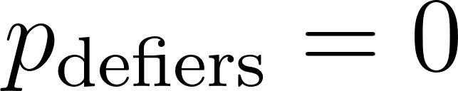The encouragement doesn’t affect the outcomes for always-takers and never-takers (exclusion restriction), i.e., .³
The encouragement works (relevance), i.e., .

With these assumptions, the formula above can be rearranged, as many terms drop out:

We have now derived the instrumental variables (IV) estimator.⁴ Again, will be undefined if there are no compliers, because then we’d divide by zero. Another way to put this is that if , then our encouragement doesn’t work, and we have no compliers by definition. If the encouragement is designed well, this, hopefully, won’t happen!

It is important to emphasize that is a local average treatment effect (LATE), and, therefore, only applies for this subpopulation. This means that if, for instance, your IV experiment had only 5% compliers, then the LATE will also only apply to these 5%, and we don’t learn anything about the treatment effect for the remaining 95% of the population. This is also the reason why IV estimators typically have higher standard errors — our statistical power only comes from a subset of the population. It is important to realize that there are compliers in both the treatment and the control groups. The compliers in the control groups are compliers in the sense that they would have taken the treatment if we had encouraged them.

An additional problem of interpretation comes from the fact that the compliers are not a well-defined population. An individual might be a complier in one experiment, but a never-taker in another closely related experiment. Whether it’s useful to make inferences about compliers is a point that is contested in the literature on instrumental variables. Making inferences about a population that is not defined beforehand but defined by the instrument itself is a weakness of the encouragement design. However, depending on the specific study, the compliers might also be exactly the population that is of interest — namely those users that we can encourage to take up a certain behavior. Either way, this difficulty of interpretation is part of the trade-off we make with encouragement designs compared to traditional A/B tests.

A closer look at the assumptions of the IV estimator

The standard assumptions that need to be satisfied in any IV study are the stable unit treatment value assumption (SUTVA) and the randomization of the treatment (here, the instrument). These are the same assumptions as in any other A/B test, so we will not delve deeper into these.

The other assumptions can be encoded in a DAG, which is shown in Figure 4.

Figure 4: a DAG diagram. — Figure 4: A DAG that shows Z as an instrumental variable. Note: Dashed lines indicate potentially unobserved relationships.

The identification problem we’re dealing with is represented by the confounders, C. Because these are typically unmeasured, we cannot simply split the sample by feature usage and learn about the causal effect of the feature D on the outcome Y. In a standard A/B test, we would randomize D, which severs the path from C to D, and identifies the causal effect. In the instrumental variable setting, however, we randomize Z.

Three assumptions around Z then need to be satisfied:

1. Monotonicity: This means that the instrument always has to work in the same direction for all individuals. Another way to state this is that there are no defiers. This assumption is probably quite plausible in many settings, or at least we can assume that the number of defiers should be fairly low. However, it is usually not too hard to tell a story where defiers are present.

2. Exclusion restriction: This assumption is visually depicted in the DAG in the sense that there is no path between Z and Y except through the feature D. Another way to state this is that the encouragement itself should not have an independent causal effect on the outcome Y. A violation of the exclusion restriction is not unlikely if the encouragement is very intrusive, especially for the never-takers who were not interested in the feature in the first place. In practice, the exclusion restriction is often the biggest issue in defending the interpretability of an IV estimate.

3. Relevance of the instrument: This is depicted in the DAG as a direct arrow between Z and D. Another way to state this is that we want feature usage to be higher in the encouraged group compared to the non-encouraged group. Luckily, this assumption is easily testable. In a broader sense, it is also important that the effect of Z on D is numerically not too small, that is, the encouragement should be substantively relevant as well. If this is not the case, you may run into the “weak instrument problem”, which can lead to large standard errors and, more seriously, to a large bias in the IV estimator. If the instrument is weak, a larger sample size can often make up for some of the weakness, however, which is good news in settings where the sample size is less of an issue. Some textbooks give the advice that the F statistic of the regression of D on Z should be at least 10, but ideally it is far larger than this.

In encouragement designs, the second and third assumptions are somewhat in opposition. On the one hand, we need to design an encouragement that is highly effective (relevant) in generating an uplift for feature usage. On the other hand, a more intrusive encouragement might also alter user behavior in unexpected ways and thereby directly influence the outcome. These two requirements need to be balanced when designing experiments with an encouragement design and, ideally, incorporate prior substantive knowledge on user behavior and encouragement effects.

If there is a concern that the exclusion restriction is not fully satisfied, it is possible to do a sensitivity analysis. For instance, one can assume a small negative effect for the never-takers (obtained, for instance, from related experiments) and test how this effect would influence the LATE.

Standard error of the IV estimator

The logic of the IV estimator is to use only part of the variance in D to estimate the treatment effect on the outcome Y. The part of the variance that we’re using is that part that is attributable to Z. However, using only part of the variance of D also means that we’ll have higher standard errors (compared to a standard A/B test).

A full derivation of the standard error of the IV estimator is outside the scope of this blog post, but the final formula is still useful to build intuition. To calculate the standard error, first define a residual. This residual is similar to the residual of a regression of Y on D, but removes only the variation that is attributable to the treatment effect of the compliers that runs through Z. For this, define as the observed value of Y for individual i, and as the observed value of D. Then, let represent the residual for the i^th individual:

where and are sample averages of and , respectively.

We can think about u_i as everything from Y that is left over after we account for the causal effect of feature usage on our outcome of interest. The variance of the IV estimator is then:

We want this quantity to be low. There are three ways to achieve this:

1. Increase the sample size, n.

2. Reduce the numerator: This is hard, because it depends on the size of , the causal effect we want to estimate. Generally, we have lower variance when our causal effect is stronger. The higher the residual variance, the harder it is to measure the effect. This is the same problem that we have in any A/B test — we need more data when we want to measure a small effect.

3. Increase the size of the denominator: The denominator measures the strength of the instrument, and will grow as the difference between and grows. If the denominator is low, we may have a “weak instrument” problem.

To make IV designs well powered, we require a large sample size and an effective instrument. Ideally, we have high feature uptake in the encouragement group, but low feature uptake in the control group.

Conclusion

Encouragement designs and IV estimators can be useful tools in situations where a standard A/B test is not possible or not desirable. The upsides of an encouragement design (allowing all users access to a feature and making marketing possible) need to be balanced with the downsides (possible violations of the exclusion restriction, the limited interpretability of the LATE, and the higher requirements to reach statistical power).

One big advantage of the encouragement design framework is that it sharpens the distinction between a feature and its entry points: the feature in itself might work very well, but only if we get it in front of the right subset of users, namely the compliers and always-takers. The total rollout impact of a feature can then be decomposed as a product of the LATE and the proportion of users using the feature, and we can think separately about optimizing each factor.

This overview of encouragement designs and IV estimation just scratches the surface of a vast literature. For instance, we assumed a binary instrument (encouraged or not encouraged) and a binary treatment (used the feature or not), but both the instrument and the treatment can also be continuous — we could think about different strengths of encouragement, for instance. A continuous instrument enables a wider range of statistical techniques. Continuous instruments, at least in theory, also allow for the estimation of heterogeneous treatment effects. Some extensions of the basic IV framework presented here are discussed in the resources given in the “Further reading” section below.

This post discussed IV estimation mostly in the context of encouragement designs, but their applicability extends beyond this context. For instance, IV estimation can be used to correct for noncompliance if there were technical problems with setting up an experiment (e.g., sample-ratio mismatch). IV estimation can also be used to estimate the causal effect of something that is difficult to manipulate directly. For instance, at Spotify we are often interested in the effects of higher consumption on different outcomes, but we can’t A/B test on consumption directly. However, if we find a valid instrument for consumption (e.g., an encouragement so that users consume more) that is not directly related to the outcome in question, then we can recover the causal effect of consumption on an outcome.

Notes

Another way to say this is that we can filter out the noncompliers of both the treatment and the control groups, which is not possible in the other two types of A/B tests. Of course, if we want to calculate the rollout impact from such an experiment, we would still need to take into account the proportion of users that use Home or Search.
We define “treated users” as users that have used the feature. However, “untreated” users might still be treated in the sense that they have seen the entry points for a feature, which might also alter their behavior. The assumption that these users are unaffected by the entry points is known as the exclusion restriction.
Saying that the ITT is zero for always-takers and never-takers does not mean that these users can’t have a treatment effect in terms of D — it just means that the encouragement doesn’t have anything to do with changing their outcome. However, it is impossible in our design to say anything about the treatment effect in terms of D for these groups as all always-takers have taken the treatment and all never-takers haven’t taken the treatment.
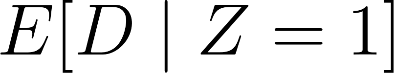
If you’re wondering about the denominator in the last expression, here’s the derivation: because of random assignment, we will have the same proportion of always-takers, never-takers, and compliers in both the “Treatment” and “Control” cells. Hence, the proportion of always-takers in our population can be estimated by E[D | Z = 0] (proportion treated in the “Control” group). Similarly, the proportion of never-takers can be estimated by 1 – E[D | Z = 1] (proportion untreated in the “Treatment” group). The proportion of compliers must be what is left over after subtracting these two groups, which is exactly what we have in the denominator.

Tags: experimentation